NOTE: This part requires some basic understanding of calculus.

These are just my solutions of the book Reinforcement Learning: An Introduction, all the credit for book goes to the authors and other contributors. Complete notes can be found here. If there are any problems with the solutions or you have some ideas ping me at bonde.yash97@gmail.com.

Grid for problems 4.1 - 4.3

4.1 Q-Values

$q_\pi(11, down) = -1 + v_\pi(T) = -1 + 0 = -1$

$q_\pi(7, down) = -1 + v_\pi(11) = -15$

4.2 state values

$v_\pi(15) = -1 + 0.25 (-20 -22-14+v_\pi(15))$

$v_\pi(15) = \frac{-15}{0.75} = -20$

No the dynamics do not change the value of the state because it is still as far off from terminal as $S_{12}$

4.3 q-value functions

$q_\pi(s,a) = \mathbb{E} \left[G_t|S_t=s, A_t=a \right]$

$q_\pi(s,a) = \mathbb{E} \left[R_{t+1} + \gamma G_{t+1} |S_t=s, A_t=a \right]$

$q_\pi(s,a) = \mathbb{E} \left[R_{t+1} + \gamma q_\pi(S_{t+1}, A_{t+1})|S_t=s, A_t=a \right]$

$q_\pi(s,a) = \sum_{s',r}p(s',r|s,a) \left[r + \gamma \sum_{a'}\pi(a'|s')q_\pi(s',a') \right]$

$q_k(s,a) = \sum_{s',r}p(s',r|s,a) \left[r + \gamma \sum_{a'}\pi(a'|s')q_{k+1}(s',a') \right]$

4.4 Subtle bug

The policy iteration algorithm has a subtle bug as follows. Imagine if we are in a state $s$ where either actions $a_1$ and $a_2$ predicted by the policy $\pi(a|s)$ lead to the same state $s'$ (assume it is terminal and there are multiple ways to reach the terminal). In this case the policy will keep on oscillating and may never terminate.

$\pi(s) \leftarrow \max_a \sum_{s',r} p(s',r|s,a) \left[r + \gamma V(s') \right] \forall s \in S$

To fix this we replace the second last line in algorithm i.e. if $\text{old action} \ne \pi(s)$ then $\text{policy-stable} \leftarrow \text{fails}$, because the policy is oscillating between equally good policies. The way to solve this is to replace it directly with the value returned, if the value is same then the policy is stable.

$\text{if } v_{\pi'}(s) = v_\pi ; \text{policy-stable} \leftarrow \text{true}$

4.5 Action Value Algorithm

The problem is to convert the policy iteration algorithm's $v_*$ to $q_*$. This can be done by adding an inner loop $\forall a \in A_s$ in 2. Policy Evaluation

$q(s,a) \leftarrow Q(s,a)$

$Q(s,a) \leftarrow \sum_{s',r}p(s'r|s,a)\left[r + \gamma \sum_{a'} \pi(a'|s') Q(s',a') \right]$

$\Delta \leftarrow \max_a \left[ \Delta, |q(s,a) - Q(s,a)| \right]$

4.6 Epsilon-soft policy

The problem is to optimize the policy iteration algorithm's when the policy is epsilon-soft i.e. minimum probability of any action is $\epsilon / |A(s)|$, thus we can modify Policy Evaluation piece as

$v(s) \leftarrow V(s)$

$a \leftarrow \max{(\epsilon / |A(s)|, \pi(s))}$

$V(s) \leftarrow \sum_{s',r}p(s'r|s,a)\left[r + \gamma V(s')\right]$

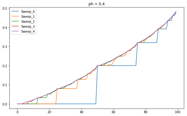
4.8 Gambler's Problem - 1

The reason it bets all the money at 50 is because that is the price at which it has the highest probability to win. If the value function represents the probability then it has highest probability of winning at 50.

Value Distribution for $p_h=0.4$

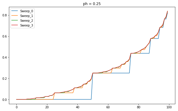
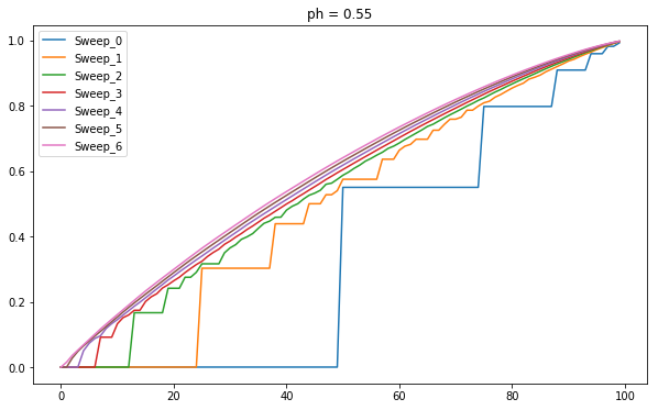
4.9 Gambler's Problem - 2

The reason it bets all the money at 50 is because that is the price at which it has the highest probability to win. If the value function represents the probability then it has highest probability of winning at 50.

Value Distribution for $p_h=0.25$

Value Distribution for $p_h=0.55$

No the results are not stable as $\theta \rightarrow 0$ as the $\Delta$ value starts to increase and learning deteriorates. I am unable to generate the optimal policies, I suspect it is because of the float values.